NLP Application: Tensorflow.js vs Tensorflow Python – Part 2

The first part demonstrated how to read in and prepare datasets. In addition, the tokenisation of a dataset was discussed in detail. The points were illustrated using an example in Tensorflow (Python) and Tensorflow.js (Tfjs). In both the Python example and the JavaScript example, the model is only able to recognise words that have occurred at least once in the data set. This model has issues with new words, because we didn’t take an OOV token into account for our NLP tensorflow application.

You might also be interested in: NLP application part 1 (reading data, preparing data and tokenisation)

OOV Token

With a translator, it is only a matter of time before an unknown word is entered. This can be a personal name, a spelling mistake or something similar. It is therefore advisable to train the model with regard to unknown words. An OOV token is needed for this. OOV stands for “out of vocabulary”. During training, the model learns to generate this token or to handle it accordingly. In this case, an unknown word can be replaced by the token “<oov>” before it is passed to the model. The model will then treat it like any other token and generate a response based on its learned behaviour.

Now you might ask how do you include this OOV token in the training data? I do this by automatically searching my dataset at the beginning for words that occur only 1 time. Then I replace these rare words with “<oov>” so that my model can also learn to react to unknown words.

Padding

In many machine learning models, including neural networks, the inputs are expected to have a fixed size or shape. This requirement arises from the structure and operation of the underlying computational graph. Inputs of the same length simplify the data processing pipeline and enable efficient batch processing.

Why the inputs should have equal length:

1. Matrix operations: Neural networks typically process inputs in batches, and batch processing is most efficient when the input data has a uniform shape. The data is organised into matrices, with each row representing an input instance. To perform matrix operations efficiently, all input instances must have the same shape.
2. Sharing of parameters: In many neural network architectures, model parameters (weights) are shared across different parts of the input sequence. For example, in recurrent neural networks (RNNs), the same weights are used to process each time step. To enable sharing of parameters, all input sequences must have the same length.
3. Memory allocation: Neural networks often allocate memory based on the maximum length of the input sequences. If the sequences have different lengths, dynamic memory allocation is required, which can be more complex and less efficient.

While it is possible to process variable length inputs using techniques such as padding and masking, this increases the complexity of the model and may require additional processing steps. For simplicity and efficiency, it is therefore common to pad or truncate sequences to a fixed length before feeding them into a neural network model.

from keras.utils import pad_sequences

# pad sequences
encoder_seq = pad_sequences(encoder, maxlen=max_encoder_sequence_len, padding="post")
decoder_inp = pad_sequences([arr[:-1] for arr in decoder], maxlen=max_decoder_sequence_len, padding="post")
decoder_output = pad_sequences([arr[1:] for arr in decoder], maxlen=max_decoder_sequence_len, padding="post")
print(encoder_seq)
print([idx_2_txt_encoder[i] for i in encoder_seq[0]])
print([idx_2_txt_decoder[i] for i in decoder_inp[0]])
print([idx_2_txt_decoder[i] for i in decoder_output[0]])

I have added the 4 print commands for better illustration. Initially, I thought that the longest record in the data set would set the length for input data and output data. So the padding length for input and output would be the same. But that is not the case! Input data and output data are normalised to different lengths!

In the example here, I have used a tiny data set where the longest English sentence consists of 3 words and the longest French sentence consists of 10 words. Accordingly, each training set is padded with “<pad>” or 0 until the input reaches 3 words and the output 10 words.

The decoder output with [arr[1:] for arr in decoder] removes the “start” token and the decoder input with [arr[:-1] for arr in decoder] removes the “end” token.

In sequence-to-sequence models, the decoder is trained to generate the output sequence based on the input sequence and the previously generated tokens. During training, the input sequence of the decoder contains the “start” token, which serves as the initialisation token for the decoder. However, when training the decoder, it is supposed to predict the next token based on the previously generated tokens, except for the “start” token. Therefore, when preparing the decoder output sequence, the “start” token is removed from each sequence. This is done to correctly match the decoder input and output sequences. The decoder input sequence contains the “Start” token and excludes the “End” token, while the decoder output sequence contains the “End” token and excludes the “Start” token. In this way, we ensure that the decoder learns to generate the correct output sequence based on the input.

During inference (model application after training) or when using the trained model to generate translations, we can start with the “start” token and iteratively generate tokens until we encounter the “end” token or reach a maximum sequence length.

When padding for Tensorflow.js, we adopt Python’s approach 1:1. Unfortunately, we again have more work and more code lines, as there is no padSequences function in Tfjs. I have therefore written my own padSequences function:

function padSequences(sequences) {
  const paddedSequences = [];
  const maxlen = findMaxLength(sequences);

  for (const sequence of sequences) {
    if (sequence.length >= maxlen) {
      paddedSequences.push(sequence.slice(0, maxlen));
    } else {
      const paddingLength = maxlen - sequence.length;
      const paddingArray = new Array(paddingLength).fill(0);
      const paddedSequence = sequence.concat(paddingArray);
      paddedSequences.push(paddedSequence);
    }
  }

  return paddedSequences;
}

We can then use this function to determine our encoder, decoder input and decoder output:

function pad(data) {
  const encoderSeq = padSequences(data.en);
  const decoderInp = padSequences(data.de.map((arr) => arr.slice(0, -1))); // Has startToken
  const decoderOutput = padSequences(data.de.map((arr) => arr.slice(1))); // Has endToken
  console.log(decoderInp);
}

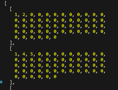
In my case, the “1” is the “startToken”, so the decoder input looks like this, for example:

Create a model

# Design LSTM NN (Encoder & Decoder)
# encoder model
encoder_input = Input(shape=(None,), name="encoder_input_layer")
encoder_embedding = Embedding(num_encoder_tokens, 300, input_length=max_encoder_sequence_len, name="encoder_embedding_layer")(encoder_input)
encoder_lstm = LSTM(256, activation="tanh", return_sequences=True, return_state=True, name="encoder_lstm_1_layer")(encoder_embedding)
encoder_lstm2 = LSTM(256, activation="tanh", return_state=True, name="encoder_lstm_2_layer")(encoder_lstm)
_, state_h, state_c = encoder_lstm2
encoder_states = [state_h, state_c]

# decoder model
decoder_input = Input(shape=(None,), name="decoder_input_layer")
decoder_embedding = Embedding(num_decoder_tokens, 300, input_length=max_decoder_sequence_len, name="decoder_embedding_layer")(decoder_input)
decoder_lstm = LSTM(256, activation="tanh", return_state=True, return_sequences=True, name="decoder_lstm_layer")
decoder_outputs, _, _ = decoder_lstm(decoder_embedding, initial_state=encoder_states)
decoder_dense = Dense(num_decoder_tokens+1, activation="softmax", name="decoder_final_layer")
outputs = decoder_dense(decoder_outputs)

model = Model([encoder_input, decoder_input], outputs)

The code example shows the design of a neural network with Long Short-Term Memory (LSTM) for sequence-to-sequence learning (Seq2Seq), which is typically used for tasks such as machine translation. The code defines two main parts: Encoder Model and Decoder Model.

Encoder Model:

• • The encoder input layer (encoder_input) represents the input sequence of the encoder model.
  • The input sequence is embedded using an embedding layer (encoder_embedding) that converts each token into a dense vector representation.
  • The embedded sequence is then passed through the first LSTM layer (encoder_lstm_1_layer) to capture sequential information. The LSTM layer returns the output sequence and the final hidden state.
  • The output sequence of the first LSTM layer is further processed by the second LSTM layer (encoder_lstm_2_layer). The second LSTM layer only returns the final hidden state, which is the summarised information of the input sequence.
  • The final hidden state of the second LSTM layer is split into the final hidden state (state_h) and the final cell state (state_c), which are used as initial states for the decoder model.
  • The states of the encoder model are defined as encoder_states and are passed on to the decoder model.

Decoder Model:

• The decoder input layer (decoder_input) represents the input sequence of the decoder model, which consists of the target sequence shifted by one position.
• Similar to the encoder, the input sequence is embedded using an embedding layer (decoder_embedding).
• The embedded sequence is then passed through an LSTM layer (decoder_lstm_layer), where the initial states are set to the final states of the encoder model. This allows the decoder to take into account the relevant information from the encoder.
• The LSTM layer provides the output sequence and the end states.
• The output sequence from the LSTM layer is passed through a dense layer (decoder_final_layer) with a softmax activation function that predicts the probability distribution over the output tokens.

The Model class is used to create the overall model by specifying the input layers ([encoder_input, decoder_input]) and the output layer (outputs). This model architecture follows the basic structure of an encoder-decoder model using LSTMs, where the encoder processes the input sequence and generates the context vector (final hidden state), which is then used by the decoder to generate the output sequence.

The same model can also be implemented in JS:

function createModell(
  numEncoderTokens,
  numDecoderTokens,
  maxEncoderSequenceLen,
  maxDecoderSequenceLen
) {
  // Encoder model
  const encoderInput = tf.input({ shape: [null], name: "encoderInputLayer" });
  const encoderEmbedding = tf.layers
    .embedding({
      inputDim: numEncoderTokens,
      outputDim: 300,
      inputLength: maxEncoderSequenceLen,
      name: "encoderEmbeddingLayer",
    })
    .apply(encoderInput);
  const encoderLstm = tf.layers
    .lstm({
      units: 256,
      activation: "tanh",
      returnSequences: true,
      returnState: true,
      name: "encoderLstm1Layer",
    })
    .apply(encoderEmbedding);
  const [_, state_h, state_c] = tf.layers
    .lstm({
      units: 256,
      activation: "tanh",
      returnState: true,
      name: "encoderLstm2Layer",
    })
    .apply(encoderLstm);
  const encoderStates = [state_h, state_c];

  // Decoder model
  const decoderInput = tf.input({ shape: [null], name: "decoderInputLayer" });
  const decoderEmbedding = tf.layers
    .embedding({
      inputDim: numDecoderTokens,
      outputDim: 300,
      inputLength: maxDecoderSequenceLen,
      name: "decoderEmbeddingLayer",
    })
    .apply(decoderInput);
  const decoderLstm = tf.layers.lstm({
    units: 256,
    activation: "tanh",
    returnState: true,
    returnSequences: true,
    name: "decoderLstmLayer",
  });
  const [decoderOutputs, ,] = decoderLstm.apply(decoderEmbedding, {
    initialState: encoderStates,
  });
  const decoderDense = tf.layers.dense({
    units: numDecoderTokens + 1,
    activation: "softmax",
    name: "decoderFinalLayer",
  });
  const outputs = decoderDense.apply(decoderOutputs);

  const model = tf.model({ inputs: [encoderInput, decoderInput], outputs });
  return model;
}

Train and save a model

# train model
loss = tf.losses.SparseCategoricalCrossentropy()
model.compile(optimizer='rmsprop', loss=loss, metrics=['accuracy'])
callback = tf.keras.callbacks.EarlyStopping(monitor='loss', patience=3)
history = model.fit(
   [encoder_seq, decoder_inp],
   decoder_output,
   epochs=80,  # 80
   batch_size=450,  # 450
   # callbacks=[callback]
)

The model.fit() function is used to train the model. The training data consists of the encoder input sequences (encoder_seq), the decoder input sequences (decoder_inp) and the decoder output sequences (decoder_output). The training is carried out for a certain number of epochs and a batch size of 450. The training progress can be monitored with the EarlyStopping callback, which stops the training if the loss has not improved after a certain number of epochs. The training progress is stored in the variable history.

The model in Tensorflow can handle both tensors and numpy arrays as inputs. If you pass numpy arrays as inputs to the fit function in TensorFlow, it will automatically convert them to tensors internally before training is performed. In the code, the encoder_seq, decoder_inp and decoder_output arrays are automatically converted to tensors when passed to the fit function. This allows TensorFlow to perform the necessary calculations during the training process.

Similarly, the fit function in TensorFlow.js can handle both tensors and arrays. So you can directly pass your 2D array (encoderSeq) as the first input and TensorFlow.js will internally convert them into tensors for training. Although you pass arrays instead of tensors, TensorFlow and TensorFlow.js are able to handle the conversion internally and perform the training accordingly.

# save model
model.save("./model-experimental/Translate_Eng_FR.h5")
model.save_weights("./model-experimental/model_NMT")

It is common to store the weights of a trained model separately from the model architecture. Storing the weights and the architecture separately allows more flexibility when loading and using the model. For example, one can load only the weights if the model architecture has been defined elsewhere or if the weights are to be used in another model with a similar architecture.

Finally, also the code in JavaScript:

async function trainModel(data) {
  const encoderSeq = padSequences(data.en);
  const decoderInp = padSequences(data.de.map((arr) => arr.slice(0, -1))); // Has startToken
  const decoderOutput = padSequences(data.de.map((arr) => arr.slice(1))); // Has endToken

  data.model.compile({
    optimizer: "rmsprop",
    loss: "sparseCategoricalCrossentropy",
    metrics: ["accuracy"],
  });
  const history = await data.model.fit(
    [encoderSeq, decoderInp],
    decoderOutput,
    {
      epochs: 80,
      batch_size: 450,
    }
  );
}

This is where my frustration with Tensorflow.js comes in. Although each step is 1:1 the same as the step in Python, training the model in Tensorflow.js doesn’t work…. I always get an error message:

C:\Users\[...]\node_modules\@tensorflow\tfjs-layers\dist\tf-layers.node.js:23386
            if (array.shape.length !== shapes[i].length) {
                            ^

TypeError: Cannot read properties of undefined (reading 'length')
    at standardizeInputData

General loss function and optimiser

Loss functions and optimisers are key components in training a machine learning model. A loss function, also known as an objective or cost function, measures the performance of a model by quantifying the dissimilarity between predicted outputs and actual objectives. The goal of training a model is to minimise this loss function, which essentially means improving the model’s ability to make accurate predictions. The choice of loss function depends on the problem at hand. For example, in classification tasks, categorical cross entropy, binary cross entropy and softmax cross entropy are common loss functions, while in regression tasks, mean square error (MSE) and mean absolute error (MAE) are often used.

An optimiser, on the other hand, is responsible for updating the model parameters (weights and biases) during training to minimise the loss function. He determines how to adjust the parameters of the model based on the calculated gradients of the loss function with respect to these parameters. Optimisers use various algorithms and techniques to efficiently search for the optimal values of the parameters. Common optimisers include Stochastic Gradient Descent (SGD), Adam, RMSprop and Adagrad. Each optimiser has its own features and hyper-parameters that can affect the training process and the convergence speed of the model.

The choice of loss function and optimiser depends on the specific task, the model architecture and the characteristics of the data set. It is important to select appropriate loss functions and optimisers to ensure effective model training and convergence to optimal performance.

Frequently used loss functions and optimisers

Loss functions:

• Categorical cross entropy: This loss function is often used in sequence-to-sequence models for multi-class classification problems where each target word is treated as a separate class.
• Sparse categorical cross entropy: Similar to categorical cross entropy, but suitable when the target sequences are represented as sparse integer sequences (e.g. using word indices).

Optimiser:

• Adam: Adam is a popular optimiser that combines the advantages of the Adaptive Gradient Algorithm (AdaGrad) and Root Mean Square Propagation (RMSprop). It adjusts the learning rate for each parameter based on previous gradients, which contributes to faster convergence and better handling of sparse gradients.
• RMSprop: RMSprop is an optimiser that maintains a moving average of squared gradients for each parameter. It adjusts the learning rate based on the size of the gradient, allowing for faster convergence and better performance on non-stationary targets.
• Adagrad: Adagrad adjusts the learning rate individually for each parameter based on historical gradient accumulation. It performs larger updates for infrequent parameters and smaller updates for frequent parameters.

Files for download

• NLP Tensorflow.js code (model has an error!)